QuITE: Query-Based Irregular Time Series Embedding

The idea

The bottleneck in irregular time series
isn't the backbone —
it's the input embedding.

Modern multivariate time series models silently assume uniform sampling at their input layer. QuITE replaces that layer with a tiny, plug-and-play module — and the rest of the model just works on irregular data.

Problem

Existing methods trade off

Specialized IMTS architectures lose backbone flexibility. Interpolation introduces artificial values that distort dynamics.

Idea

Learnable query tokens

A single self-attention layer lets a small set of queries aggregate irregular observations into a fixed-shape embedding — like [CLS] in BERT.

Result

Drop-in gain on every backbone

Up to +54.7% MSE reduction in forecasting and +15.8% in classification, with fewer parameters than the original backbone.

Full abstract

Irregular Multivariate Time Series (IMTS) are common in practice, yet their irregular sampling complicates effective modeling. Existing approaches typically either (i) design specialized architectures that limit the reuse of proven MTS models, or (ii) map IMTS onto regular temporal grids through interpolation, which may distort temporal dynamics by introducing artificial values. To address these limitations, we propose a new input-embedding-based approach. We identify that the key bottleneck lies not in the backbone architecture, but in conventional embedding layers that assume uniform sampling. We introduce QuITE, a simple yet effective plug-and-play embedding module for IMTS that employs learnable query tokens to aggregate irregular observations through a single self-attention layer, directly producing backbone-compatible latent representations without artificial value generation or architectural modification. Extensive experiments show that QuITE consistently improves MTS models, yielding average relative gains of up to 54.7% in forecasting and 15.8% in classification across diverse datasets and backbone architectures.

Approach	No artificial value	Model flexibility
Architecture-based	✓	✗
Data-based	✗	✓
Input-embedding-based (Ours)	✓	✓

Method

Tokenize. Then aggregate.

Two stages, one self-attention layer — that's all QuITE adds to the backbone.

Figure 1. QuITE framework — irregular observations are tokenized into (time, value) embeddings, then a small set of learnable query tokens aggregate them via masked self-attention.

A

Tokenization

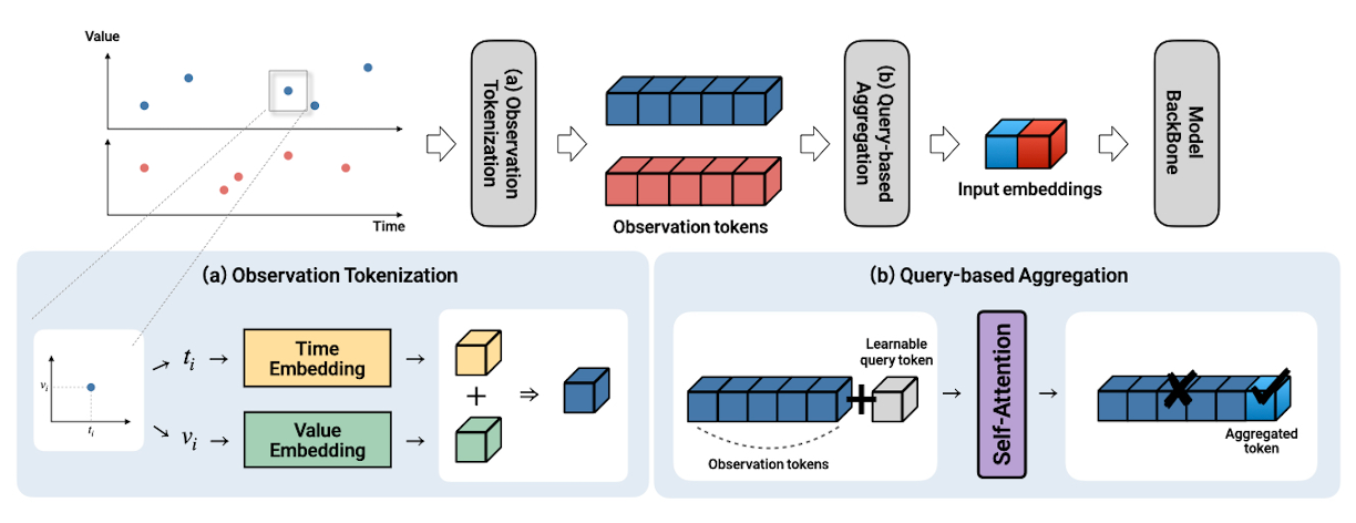
Each observation becomes one token

Every value–time–mask triplet $(x_{n,i}, t_{n,i}, m_{n,i})$ is encoded as the sum of a harmonic time embedding and a learned value projection. No interpolation — the irregular set is preserved exactly.

$$\phi(t)[k] = \begin{cases} \omega_0 t + \alpha_0, & k = 0 \\ \sin(\omega_k t + \alpha_k), & k > 0 \end{cases}$$

$$\mathbf{z}_{n,i} = f_{\text{val}}(x_{n,i}) + \phi(t_{n,i})$$

B

Aggregation

One learnable query summarizes them all

A learnable query token $\mathbf{q}_n$ is prepended to the observation tokens, and a single masked self-attention layer lets the query summarize all observed entries. Two flavors: variable-level (variate-token models) and patch-level (patch-token models).

$$\mathbf{H}_n = \text{SelfAttn}([\mathbf{q}_n;\mathbf{Z}_n],\ [1\,|\,\mathbf{m}_n])$$

$$\mathbf{e}_n = \mathbf{H}_n[0] \in \mathbb{R}^D \quad\Rightarrow\quad \mathbf{E}^{\text{var}}\in\mathbb{R}^{N\times D}$$

Extension

QuITE⁺⁺ — a forecasting architecture built natively around queries

Hierarchical encoder interleaving patch- and variable-level attention, with a cross-attention decoder over future timestamps.

Figure 2. QuITE⁺⁺ — patch-level intra-variable attention, variable-level inter-variable attention, and a cross-attention decoder.

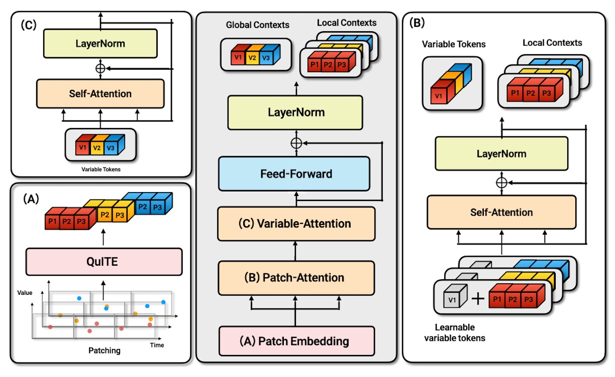
Patch-level attention

Aggregates information across temporal patches within each variable.

Variable-level attention

Models cross-variable dependencies along the variate axis.

Cross-attention decoder

Future time embeddings query the encoder for arbitrary forecast horizons.

Dataset	Samples	Vars	Avg L	Missing
Human Activity	5,400	12	120	75.0%
USHCN	26,736	5	163	77.9%
PhysioNet	12,000	36	74	88.4%
MIMIC-III	23,457	96	46	96.7%

Dataset	Samples	Vars	Classes	Missing
P19	38,803	34	2	94.9%
P12	11,988	36	2	88.4%
PAM	5,333	17	8	60.0%

Headline results

Every backbone gets better.
Every benchmark, every metric.

Six representative MTS backbones (PatchTST, PatchMixer, TMix, iTransformer, S-Mamba, TimeXer) across four forecasting and three classification benchmarks.

Forecasting MSE (lower is better)

↓ up to 54.7%

Classification score (higher is better)

↑ up to 15.8%

Forecasting MSE improvement

iTransformer

↓ 54.7%

S-Mamba

↓ 25.0%

PatchTST

↓ 16.2%

TimeXer

↓ 12.0%

TMix

↓ 11.4%

PatchMixer

↓ 5.1%

Classification gain

PatchMixer

↑ 15.8%

TMix

↑ 13.8%

S-Mamba

↑ 6.5%

PatchTST

↑ 6.3%

iTransformer

↑ 5.3%

TimeXer

↑ 5.3%

Forecasting comparison

All forecasting models, side by side.

11 IMTS-specific baselines, 6 QuITE-equipped MTS backbones, and QuITE⁺⁺ across 4 datasets × 3 horizons × MSE/MAE = 24 settings (Table 4). QuITE⁺⁺ achieves the best result in 20/24. red = best, blue = second-best.

Model	3000→1000 (ms)		2000→2000 (ms)		1000→3000 (ms)
Model	MSE	MAE	MSE	MAE	MSE	MAE
IMTS-specific baselines
Warpformer	2.61	3.12	3.60	3.81	4.26	4.26
Raindrop	4.42	4.65	5.57	5.15	5.75	5.37
GRU-D	3.94	4.37	5.93	5.66	6.14	5.75
tPatchGNN	2.79	3.24	3.71	3.89	4.56	4.32
GraFITi	3.03	3.45	4.59	4.45	4.91	4.62
CRU	3.03	3.60	4.12	4.43	4.85	4.86
mTAND	3.14	3.71	4.38	4.59	5.29	5.12
NeuralFlow	4.29	4.61	5.47	5.35	6.01	5.66
Latent-ODE	3.32	3.91	5.04	5.11	5.48	5.33
HyperIMTS	2.49	3.02	3.15	3.58	4.00	4.13
Hi-Patch	2.56	3.12	3.26	3.67	4.20	4.22
MTS + QuITE
PatchTST + QuITE	2.76	3.14	3.62	3.74	4.69	4.29
PatchMixer + QuITE	2.78	3.13	3.67	3.75	4.71	4.31
TMix + QuITE	2.77	3.15	3.66	3.74	4.75	4.38
iTransformer + QuITE	2.58	3.12	3.25	3.65	4.10	4.18
S-Mamba + QuITE	2.72	3.24	3.37	3.72	4.22	4.22
TimeXer + QuITE	2.53	3.04	3.19	3.57	4.04	4.03
QuITE⁺⁺	2.46	2.92	3.11	3.49	3.96	4.04

Model	24→1 (months)		24→6 (months)		24→12 (months)
Model	MSE	MAE	MSE	MAE	MSE	MAE
IMTS-specific baselines
Warpformer	5.09	3.10	5.12	3.13	5.10	3.13
Raindrop	5.64	3.29	7.01	4.24	7.61	4.61
GRU-D	5.17	3.21	5.29	3.34	5.36	3.25
tPatchGNN	5.00	3.07	5.23	3.24	6.23	3.83
GraFITi	5.07	2.97	5.12	3.09	5.01	3.14
CRU	5.15	3.18	6.77	4.11	6.64	4.08
mTAND	5.03	3.00	5.16	3.10	5.07	3.09
NeuralFlow	5.41	3.35	5.52	3.46	5.48	3.56
Latent-ODE	5.16	3.21	5.18	3.36	5.23	3.35
HyperIMTS	4.96	3.00	4.99	3.10	4.97	3.08
Hi-Patch	5.00	3.03	5.13	3.05	5.04	3.03
MTS + QuITE
PatchTST + QuITE	5.07	3.01	5.06	3.17	5.04	3.00
PatchMixer + QuITE	5.11	3.06	5.02	3.04	5.00	3.07
TMix + QuITE	5.18	3.10	5.52	3.39	5.03	3.05
iTransformer + QuITE	5.06	3.06	4.86	2.96	4.94	3.01
S-Mamba + QuITE	5.04	3.06	4.93	3.04	4.93	3.02
TimeXer + QuITE	4.97	2.97	4.98	3.05	4.93	2.97
QuITE⁺⁺	4.84	2.92	4.81	2.94	4.81	2.93

Model	12→36 (hours)		24→24 (hours)		36→12 (hours)
Model	MSE	MAE	MSE	MAE	MSE	MAE
IMTS-specific baselines
Warpformer	6.51	4.24	5.04	3.72	4.17	3.38
Raindrop	10.24	5.83	10.63	6.02	10.67	5.87
GRU-D	7.80	5.13	5.76	4.53	6.85	4.88
tPatchGNN	6.45	4.24	5.06	3.75	4.22	3.38
GraFITi	6.30	4.38	5.11	3.96	4.58	3.65
CRU	7.66	4.97	6.43	4.51	6.74	4.82
mTAND	7.46	4.85	6.18	4.44	5.61	4.15
NeuralFlow	7.98	5.08	7.68	4.84	8.87	5.43
Latent-ODE	7.28	4.83	6.85	4.77	6.99	4.74
HyperIMTS	6.11	4.16	4.65	3.56	3.99	3.21
Hi-Patch	6.39	4.10	5.07	3.63	4.27	3.30
MTS + QuITE
PatchTST + QuITE	17.47	7.15	10.62	5.17	8.87	4.43
PatchMixer + QuITE	17.52	7.22	11.88	5.62	9.06	4.55
TMix + QuITE	17.48	7.21	10.72	5.22	8.96	4.50
iTransformer + QuITE	6.32	4.15	4.99	3.65	4.33	3.34
S-Mamba + QuITE	6.26	4.11	5.11	3.67	4.11	3.27
TimeXer + QuITE	6.18	4.08	4.91	3.64	4.06	3.27
QuITE⁺⁺	6.08	3.99	4.99	3.62	3.81	3.18

Model	12→36 (hours)		24→24 (hours)		36→12 (hours)
Model	MSE	MAE	MSE	MAE	MSE	MAE
IMTS-specific baselines
Warpformer	2.32	8.14	1.76	7.27	1.45	6.74
Raindrop	2.36	8.63	2.31	8.61	2.21	9.17
GRU-D	2.39	8.43	2.35	8.34	2.03	8.14
tPatchGNN	2.35	8.23	1.97	7.76	1.44	6.78
GraFITi	2.22	8.13	1.76	7.28	1.61	7.16
CRU	2.34	8.32	2.23	7.99	2.00	8.16
mTAND	2.29	8.38	2.15	8.00	2.01	8.13
NeuralFlow	2.26	8.29	2.34	8.09	1.97	8.39
Latent-ODE	2.38	8.35	2.11	7.76	1.90	7.92
HyperIMTS	1.85	7.71	1.68	6.92	1.52	6.68
Hi-Patch	1.88	7.95	1.70	7.18	1.56	6.74
MTS + QuITE
PatchTST + QuITE	5.37	17.01	3.90	12.35	3.82	11.84
PatchMixer + QuITE	5.37	16.96	3.94	12.34	3.87	11.51
TMix + QuITE	5.41	16.94	3.98	12.32	3.87	11.63
iTransformer + QuITE	1.83	7.64	1.67	6.93	1.56	6.78
S-Mamba + QuITE	1.82	7.56	1.64	6.90	1.52	6.64
TimeXer + QuITE	1.84	7.67	1.68	7.12	1.55	6.73
QuITE⁺⁺	1.80	7.54	1.63	6.83	1.48	6.56

Ablation · Embedding methods

What if we replace QuITE with something simpler?

Compared against four standard input adaptations — Add, Concat, mTAND interpolation, Mean Pool — on PatchTST, iTransformer, and QuITE⁺⁺ (Table 5).

Method	Metric	PatchTST				iTransformer				QuITE⁺⁺
Method	Metric	Activity	USHCN	PhysioNet	MIMIC-III	Activity	USHCN	PhysioNet	MIMIC-III	Activity	USHCN	PhysioNet	MIMIC-III
Add	MSE	4.00	5.23	13.79	4.71	4.98	6.26	18.26	6.34	3.44	5.05	5.34	1.71
Add	MAE	4.03	3.17	6.54	14.74	4.84	3.80	8.01	19.73	3.76	3.04	3.86	7.31
Concat	MSE	3.90	5.21	12.97	4.52	5.77	6.10	18.27	6.48	3.35	4.99	5.43	1.75
Concat	MAE	3.91	3.18	5.96	14.13	5.21	3.67	8.01	20.28	3.71	3.02	3.90	7.28
mTAND	MSE	3.74	5.21	13.38	4.39	3.50	5.23	13.11	4.34	3.34	5.01	4.96	1.71
mTAND	MAE	3.76	3.20	6.03	13.80	3.65	3.15	5.96	13.72	3.64	3.07	3.60	7.17
Mean Pool	MSE	3.75	5.14	12.84	4.43	3.59	5.08	12.15	4.33	3.31	4.94	5.26	1.69
Mean Pool	MAE	3.77	3.19	5.95	13.84	3.72	3.11	5.70	13.61	3.64	3.01	3.89	7.23
QuITE	MSE	3.69	5.06	12.32	4.36	3.31	4.95	5.21	1.69	3.18	4.82	4.96	1.64
QuITE	MAE	3.72	3.06	5.58	13.73	3.65	3.01	3.71	7.12	3.48	2.93	3.60	6.98

vs. Add

12 / 12 MSE wins

vs. Concat

12 / 12 MSE wins

vs. mTAND

11 / 12 MSE wins

vs. Mean Pool

12 / 12 MSE wins

Analysis

A · Embedding quality

Tighter, more separable clusters

t-SNE projection of learned embeddings on PAM (8 activity classes). Across patch-, variable-, and hybrid-token backbones, QuITE produces more compact and clearly separated clusters.

PatchTST patch-token

w/o QuITE

w/ QuITE

iTransformer variable-token

w/o QuITE

w/ QuITE

TimeXer hybrid

w/o QuITE

w/ QuITE

Figure 4 (paper) · t-SNE Visualization on PAM

Figure 3. Additional random observation removal of 0–75% on top of already-sparse benchmarks.

B · Observation sparsity

Stable up to 50% extra missingness

On benchmarks that are already 75–97% sparse, accuracy degrades only marginally up to 50% additional removal. Even at 75% removal, the model still produces usable predictions on most datasets.

MSE across hyperparameter sweeps

Activity USHCN PhysioNet MIMIC-III

Figure 5 — all sensitivity curves are essentially flat.

C · Hyperparameter sensitivity

Robust to hyperparameter choices

Grid sweep over hidden dim ∈ {32, 64}, layers ∈ {1, 2, 3}, heads ∈ {1, 2, 4, 8} on the four forecasting benchmarks. QuITE⁺⁺ remains generally robust across different hyperparameter choices.

D · Query initialization

Robust to initialization

QuITE remains robust across initialization schemes (Xavier / Uniform / Zero / Random), with only minor performance differences.

Dataset	Metric	Xavier	Uniform	Zero	Random
Activity 3000→1000	MSE	2.46	2.45	2.46	2.46
Activity 3000→1000	MAE	3.00	2.99	3.01	2.92
USHCN 24→12	MSE	4.83	4.86	4.87	4.81
USHCN 24→12	MAE	2.99	2.95	2.98	2.93

E · Computational efficiency

Favorable accuracy–complexity trade-off

Computationally, QuITE-equipped models often used fewer parameters and generally reduced FLOPs compared to their base counterparts, indicating a favorable accuracy–complexity trade-off.

PhysioNet 24h → 24h · excerpted from Tables E.1–E.2

Backbone	Params	FLOPs	MSE
PatchTST	1.73M	75.2G	15.28
+ QuITE	127K	10.6G	10.62
iTransformer	1.77M	107G	16.48
+ QuITE	129K	13.8G	4.99
S-Mamba	2.52M	63.2G	6.93
+ QuITE	190K	8.5G	5.11

Conclusion

Bridging irregular data and proven backbones.

QuITE offers a powerful and flexible input-embedding module that bridges the gap between irregular time series data and existing, validated MTS backbones — enabling their effective application to challenging IMTS tasks without architectural modifications or artificial value generation. By aggregating irregular observations through learnable query tokens at the input stage, QuITE preserves backbone flexibility while avoiding the distortion of interpolation. Built on the same principle, QuITE⁺⁺ extends this idea into a full hierarchical forecasting architecture and achieves the best result in 20 out of 24 settings across diverse IMTS benchmarks.

Cite this work

BibTeX

@inproceedings{lim2026quite,
  title     = {QuITE: Query-Based Irregular Time Series Embedding},
  author    = {Lim, JungHoon},
  booktitle = {Proceedings of the 43rd International Conference on Machine Learning (ICML)},
  year      = {2026}
}

Correspondence: junghoon9502@gmail.com

Acknowledgements

We thank Daheen Kim and Seunghan Lee for insightful discussions and feedback. We are also grateful to Prof. Changhee Lee, Dr. Jaeho Kim, Seongjun Lee, and Seokhyun Lee of Korea University, and Prof. Kyungwoo Song of Yonsei University. Finally, we thank the anonymous ICML reviewers for their constructive comments.

QuITE: Query-Based
Irregular Time Series Embedding

The bottleneck in irregular time series
isn't the backbone —
it's the input embedding.

Existing methods trade off

Learnable query tokens

Drop-in gain on every backbone

Two existing camps, each with a cost.

Build a new model for IMTS

Resample to a regular grid

Replace the input embedding

Tokenize. Then aggregate.

Each observation becomes one token

One learnable query summarizes them all

QuITE⁺⁺ — a forecasting architecture built natively around queries

Patch-level attention

Variable-level attention

Cross-attention decoder

Seven IMTS benchmarks across three domains.

Every backbone gets better.
Every benchmark, every metric.

All forecasting models, side by side.

What if we replace QuITE with something simpler?

Tighter, more separable clusters

Stable up to 50% extra missingness

Robust to hyperparameter choices

Robust to initialization

Favorable accuracy–complexity trade-off

Bridging irregular data and proven backbones.

BibTeX

The bottleneck in irregular time seriesisn't the backbone — it's the input embedding.

Existing methods trade off

Learnable query tokens

Drop-in gain on every backbone

Two existing camps, each with a cost.

Build a new model for IMTS

Resample to a regular grid

Replace the input embedding

Tokenize. Then aggregate.

Each observation becomes one token

One learnable query summarizes them all

QuITE++ — a forecasting architecture built natively around queries

Patch-level attention

Variable-level attention

Cross-attention decoder

Seven IMTS benchmarks across three domains.

Every backbone gets better.Every benchmark, every metric.

All forecasting models, side by side.

What if we replace QuITE with something simpler?

Tighter, more separable clusters

Stable up to 50% extra missingness

Robust to hyperparameter choices

Robust to initialization

Favorable accuracy–complexity trade-off

Bridging irregular data and proven backbones.

BibTeX

The bottleneck in irregular time series
isn't the backbone —
it's the input embedding.

QuITE⁺⁺ — a forecasting architecture built natively around queries

Every backbone gets better.
Every benchmark, every metric.